Machine Learning on Databricks for Data Engineers

I built two models on Databricks from scratch — one predicts a used bike's price, and one predicts whether a loan will default. Both follow the same pattern: raw file → feature table → training → saved model → predictions. The useful lesson came from the loan model: nearly 90% accuracy sounded good, but the model caught almost none of the defaults. Accuracy alone hid the result that mattered.

TL;DR

• Two models on a fake e-bike shop dataset: price (regression) and loan default (classification).

• Linear Regression had the lowest held-out MAE for price - with only 817 usable bikes, the simple model performed best on the primary KPI.

• The default classifier was close to 90% accurate but caught only about 1% of defaults.

• Retraining with class balancing lowered accuracy but caught roughly 70% of defaults.

• The worked example at the end explains why accuracy is not enough when the important rows are rare.

The method, end to end

Every model in this project follows the same six steps. each phase below maps back to it:

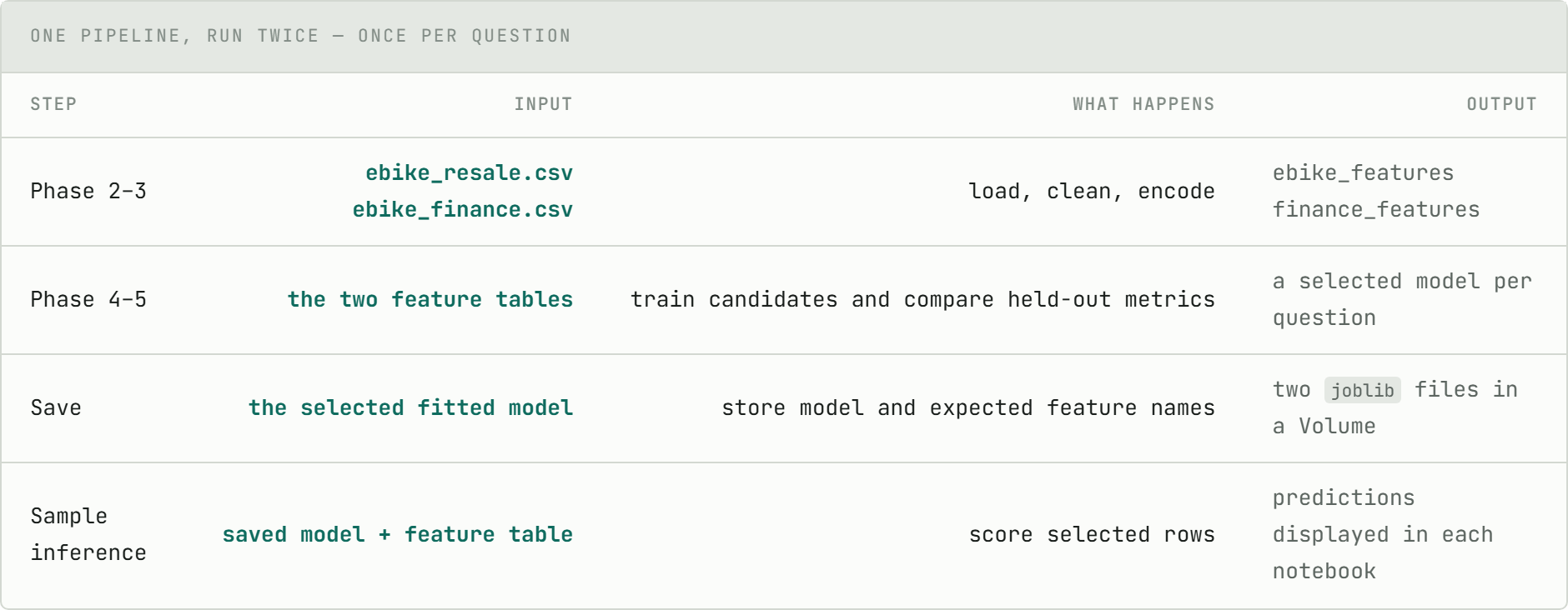
Two questions, one pipeline shape. What will this bike sell for? → regression (Phase 4). Will this loan default? → classification (Phase 5). Same steps, run twice.

Phase 1 · What a model actually is

A model is a function learned from historical examples instead of a set of rules written by hand.

You show it past rows where you already know the answer ,this bike sold for £2,000, that one for £500 ;and it finds a pattern. For a new row, it applies that pattern. In code, that's it:

model.fit(examples, answers)     # here's what happened before
model.predict(new_case)          # now guess this one

Supervised = you have the answer column already (paid back or not).

Unsupervised = no answer column, just "find groups" or "find weird rows." This project is supervised only.

A data engineer may not choose the final algorithm, but still needs to understand what goes into it, what comes out, and how it will run in production.

The model families used in this project

These are the model families the notebooks actually compare:

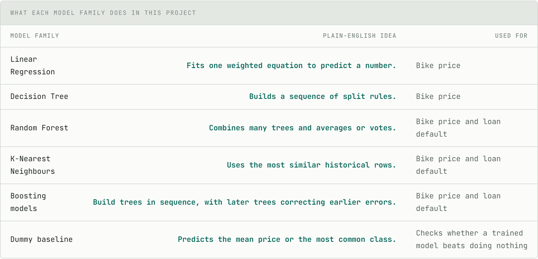
K-Means, DBSCAN and Isolation Forest are useful unsupervised tools, but they are not part of these two Pedalflow pipelines, so they are outside this walkthrough.

Regression vs classification - The rule that saves you

"Regression" means number. "Classification" means yes/no. Except Logistic Regression, which does yes/no despite the name .

Both Linear and Logistic Regression sum weighted inputs. Linear outputs a number. Logistic squashes the sum to 0–1 so it reads as a probability.

The one rule that actually matters

Look at the target column, not the algorithm name. 
Number target → regression. Yes/no target → classification.

predicted_price_gbp could be 1432.57, so it is regression. The loan result is class 0 or 1, so it is classification. The associated probability tells us how strongly the model leans toward class 1.

You pick the question by picking the target column. The algorithm follows.

Phase 2 · Meet Pedalflow

You are here: raw CSVs. Nothing cleaned yet.

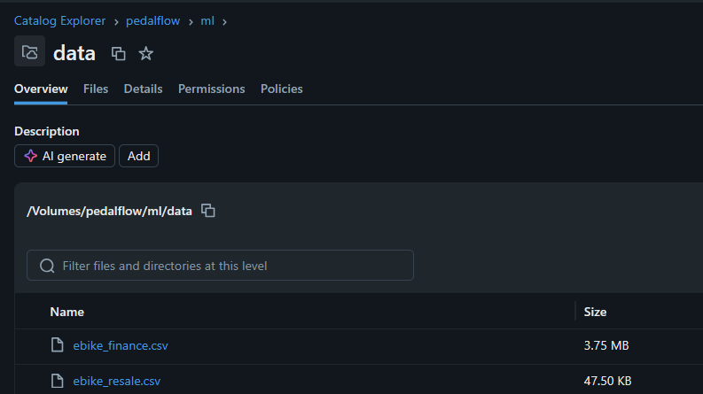
Pedalflow is a fake e-bike shop I made up for this walkthrough. Two datasets: used-bike resale (regression) and loan applications/ebike_finance (classification).

Spreadsheet 1: a used bike for sale

One row = one bike. Target: Resale_Price_GBP.

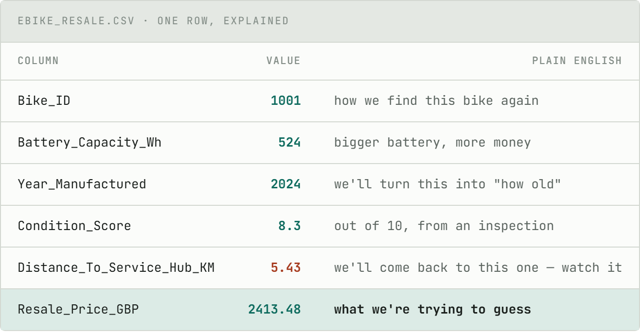
Nearly new, good condition, sold for £2,413. Across the file, prices run from £120 to about £11,000, with a typical bike around £1,174.

Spreadsheet 2: someone asking to finance a bike

One row = one loan application, captured before approval. Target: IsDefault (0 = paid, 1 = defaulted). Every feature must be knowable at decision time — no future payment history.

~10% of loans default. That imbalance drives everything in Phase 5.

All data is synthetic and generated from a fixed seed. The raw rows are reproducible, but exact model metrics can still move with library versions and time-dependent features such as Bike_Age, which the notebook calculates from the current year.Phase 3 · Loading and cleaning the data

Bike file (regression)

Load — nothing new if you read CSVs for a living:

df = spark.read.csv("ebike_resale.csv", header=True, inferSchema=True)

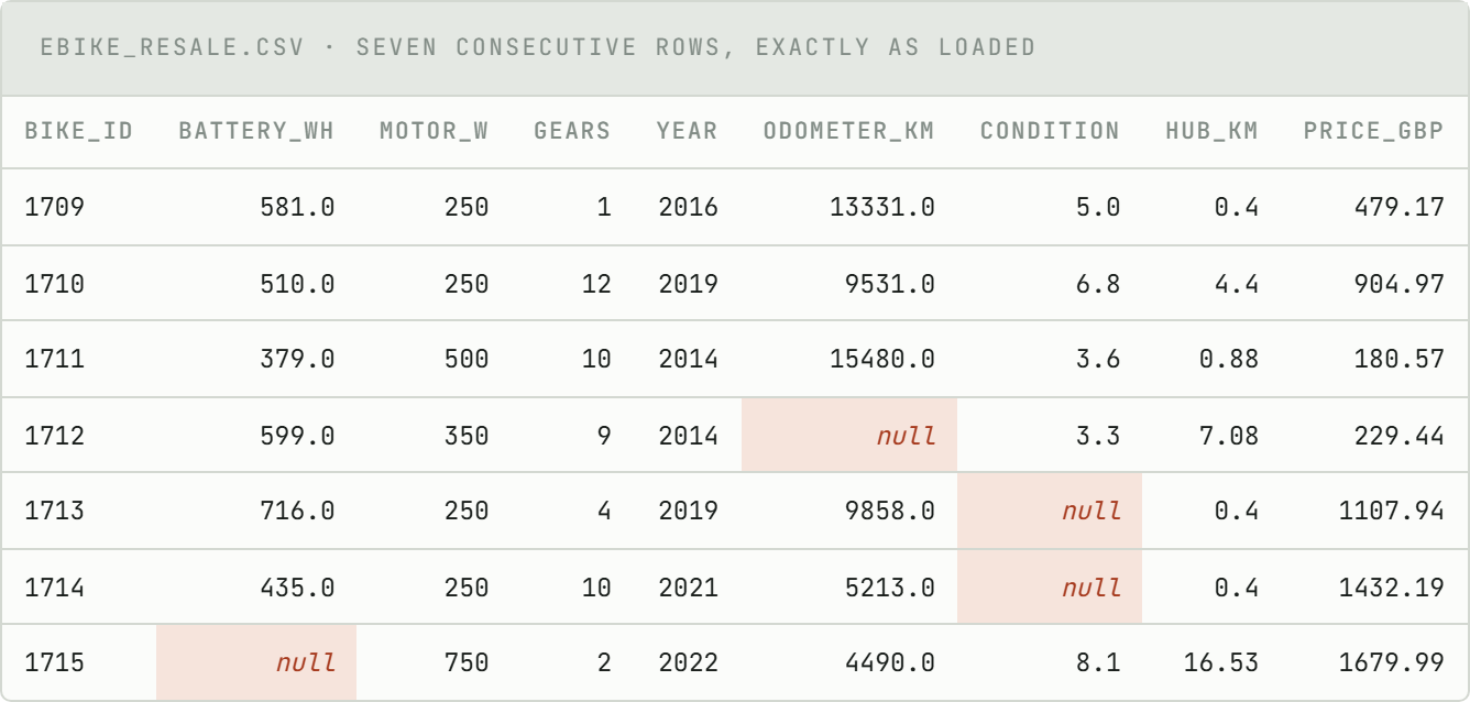
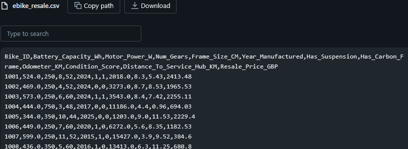
900 bikes in, blanks and all. Four gaps in seven rows - and those blanks are the next decision.

Three cleaning steps:

1. Nulls. Four gaps in seven sample rows. Easy fix: dropna() — 900 rows become 817. But first check: are nulls random, or do cheap bikes skip inspection? Dropping blindly can bias the training set.

900 rows in → 817 rows saved → 83 rows dropped for missing values.

One line of code, nine per cent of the data gone. Saved as pedalflow.ml.ebike_features so every later step reads the same 817 rows.

1. Feature engineering. Replaced Year_Manufactured with Bike_Age. "Made in 2019" is weak; "7 years old" is useful. Domain knowledge beats algorithm choice here.

2. Scaling. Battery capacity is in hundreds, while gears are under 20. This matters for distance-based models such as KNN and can matter for some linear or gradient-based models. Tree models are much less sensitive to scale. Dividing each numeric column by its standard deviation keeps the comparison fair across the model families used here.

Evaluation limitation

The current notebook calculates standard deviations before the train/test split. That lets the held-out data influence preprocessing slightly. A production pipeline should fit scaling parameters on the training rows only, then reuse those exact parameters for test and inference data.

No text columns in this file - no encoding needed. The target column (Resale_Price_GBP) stays out of the feature table.

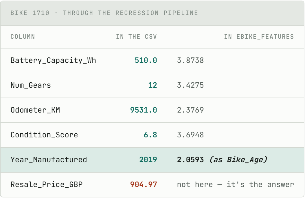
Scaled values aren't human-readable - that's fine. The model doesn't need pounds and years; it needs consistent numbers.

Result: 817 rows, 11 columns, saved as pedalflow.ml.ebike_features.

Loan file (classification)

df = spark.read.csv("ebike_finance.csv", header=True, inferSchema=True)

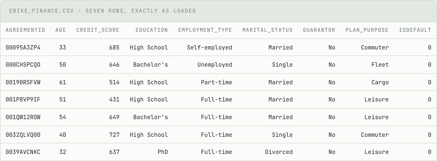
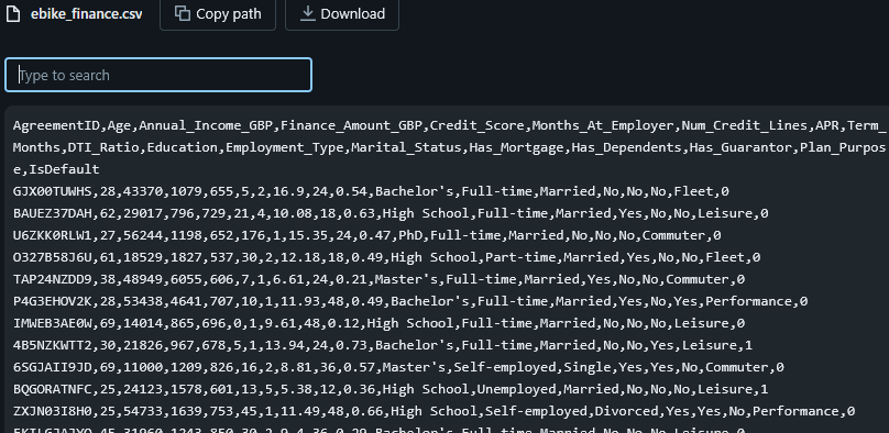
Six of the nine columns here are words, and not one of them means anything to a model until it becomes a number. IsDefault is the answer we're trying to learn - 0 means they paid.

Different problems:

1. Nulls: none. Same dropna() line, zero rows lost. Don't drop nulls by reflex — check first.

2. No scaling, no new columns in this notebook.

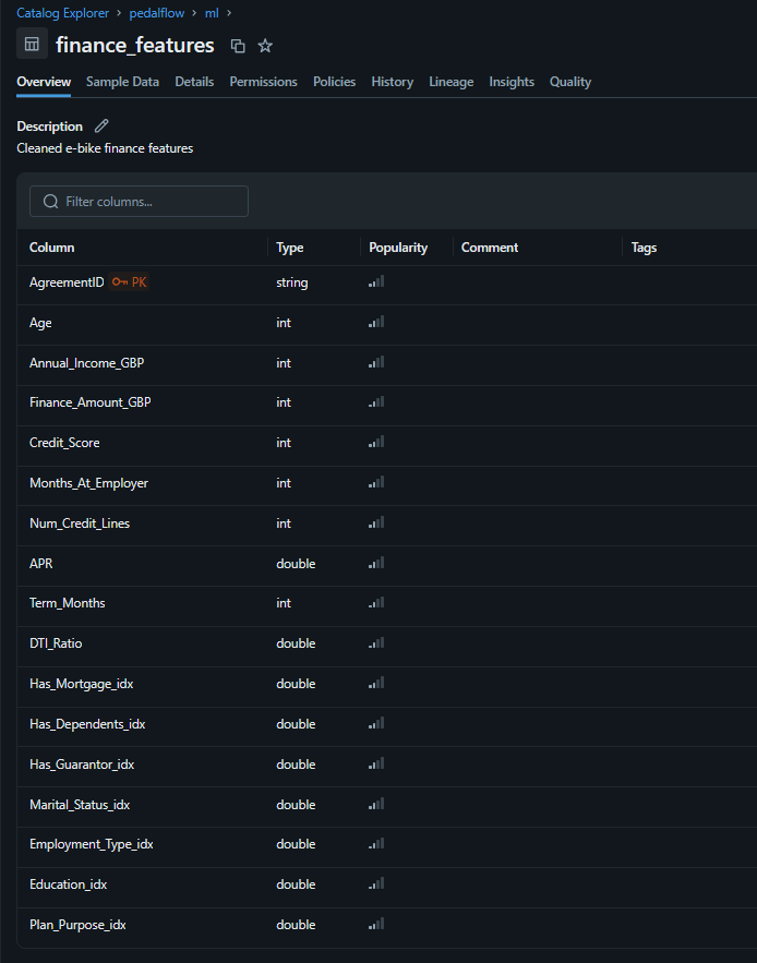
3. Encoding: seven text columns → numbers. Models do arithmetic, not English.

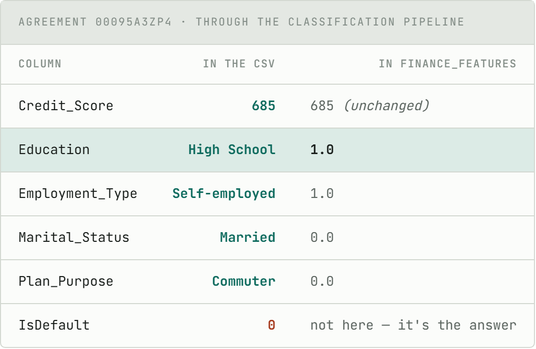
What do 0, 1, 2 and 3 mean? They are category codes, not weights or scores. For example, the notebook currently maps Married, Single and Divorced to three numbers based on how often each value appears. A code of 2 does not mean “twice as important” as a code of 1.

There is one important catch: scikit-learn receives these columns as ordinary numbers. A Random Forest can therefore split a column with a rule such as Marital_Status_idx <= 1.5. That introduces an artificial order even though marital status has no natural ranking. The numbers are intended as IDs, but the current models can still use their numeric order.

A limitation in the current notebook

The frequency encoding is a convenient demo shortcut, not the design I would use in production. Education should use an explicit order. Unordered columns such as employment type, marital status and plan purpose should normally use one-hot encoding, or a model configured to handle categorical values directly. The mapping should be fitted on training data, saved and reused so test data cannot influence it and new data cannot silently change the codes.

Binary Yes/No columns can safely use a fixed 0/1 mapping. Existing numeric columns such as age, income and credit score stay numeric. The target, IsDefault, is kept out of the feature table.

The loan notebook does not scale its numeric features. That is acceptable for the tree-based models, but it puts KNN at a disadvantage because large-range columns such as income dominate its distance calculation. Treat the KNN result as illustrative unless it is rerun with suitable preprocessing.

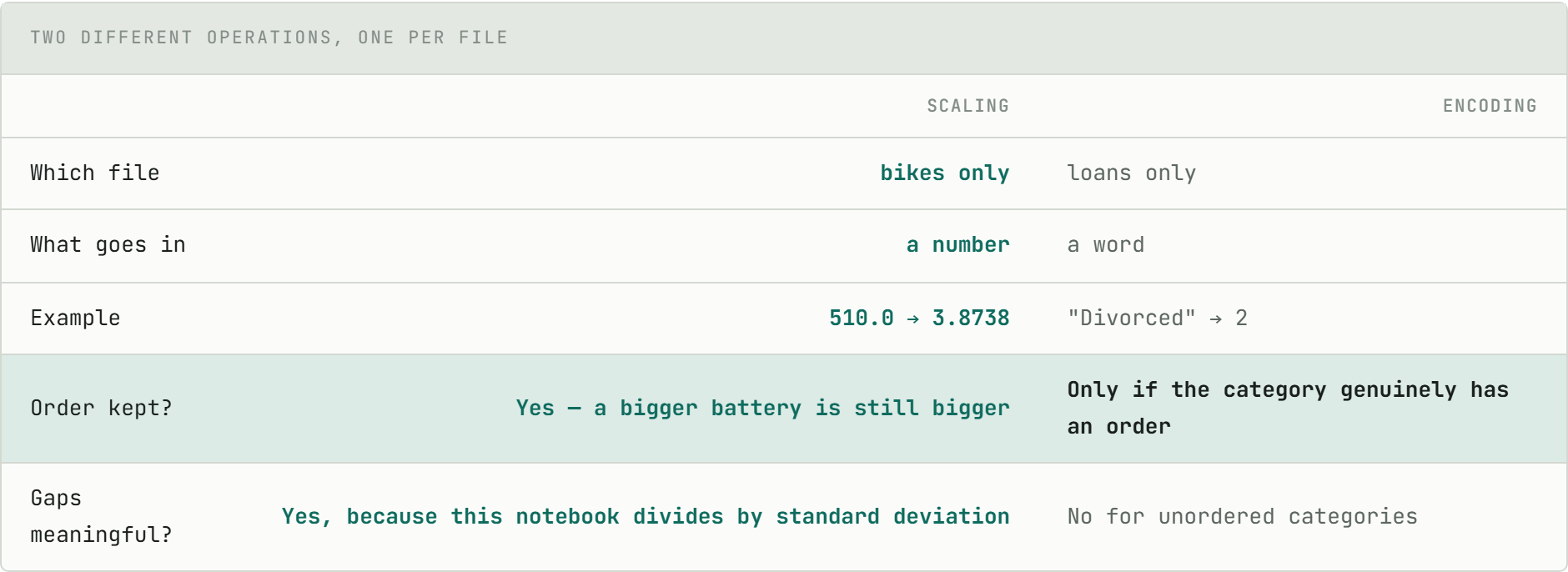
Scaling ≠ encoding

Scaling (bikes): shrinks numbers, keeps order. Encoding (loans): assigns arbitrary integers to categories. Different operations, different files.

Words became numbers; the label stayed out. Output: 40,000 rows → pedalflow.ml.finance_features.

The two side by side

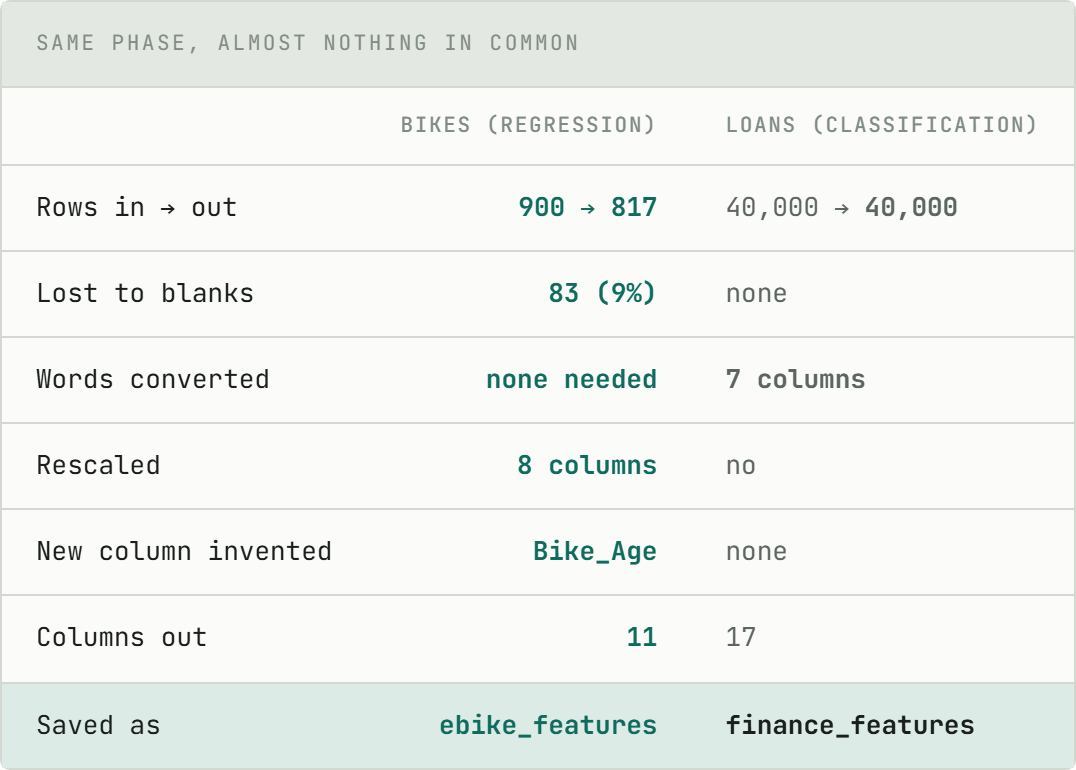
Save feature tables to Unity Catalog - not notebook variables. Training and scoring must read identical columns built the same way, or the model drifts silently.

Phase 4 · Train: predict bike price

You are here: ebike_features → pick a winning regressor.

The feature table deliberately excludes the answer. The training notebook reads Bike_ID and Resale_Price_GBP from the source file, then uses a Databricks FeatureLookup to join those labels back to ebike_features by Bike_ID. The loan notebook follows the same pattern with AgreementID and IsDefault.

How do you measure error on rows you haven't seen?

Hold out a test set. Same idea as validating a pipeline against a known-good sample:

817 bikes, all with known sale prices
  |
  +-- 653 bikes  TRAINING   model sees the prices, learns from them
  |
  +-- 164 bikes  TESTING    prices hidden from the model completely

653 train, 164 test. Model never sees test labels during training. Loans split 32k/8k with stratify=y so ~10.6% default rate holds in both halves.

Regression KPIs: how we choose the best price model

In ML these are usually called evaluation metrics. From a delivery point of view, they are the KPIs used to decide whether one model is better than another. The primary KPI should be chosen from the business problem before comparing models; otherwise it is easy to pick whichever number makes a preferred model look good.

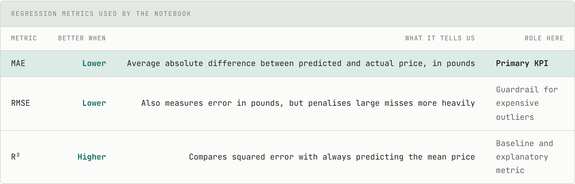
Why MAE is primary: the business question is “how many pounds away was the estimate?” MAE answers that directly and gives equal importance to overpricing and underpricing. RMSE is checked as a guardrail because the dataset contains a few high-value collector bikes, where a large miss matters. R² confirms that the model adds value over a simple mean-price baseline.

Selection rule: compare every model on the same 164 held-out bikes, select the lowest MAE, then confirm that RMSE is acceptable and R² is positive. Using that rule, Linear Regression is the selected model for this run.

Why MAE is primary: the business question is “how many pounds away was the estimate?” MAE answers that directly and gives equal importance to overpricing and underpricing. RMSE is checked as a guardrail because the dataset contains a few high-value collector bikes, where a large miss matters. R² confirms that the model adds value over a simple mean-price baseline.

Selection rule: compare every model on the same 164 held-out bikes, select the lowest MAE, then confirm that RMSE is acceptable and R² is positive. Using that rule, Linear Regression is the selected model for this run.

Seven tools, same 817 bikes

Train seven algorithms, log metrics to MLflow - same loop as any batch job you'd audit later:

model_variants = {
    "Linear Regression": LinearRegression(),
    "Decision Tree": DecisionTreeRegressor(),
    "Random Forest": RandomForestRegressor(),
    "XGBoost": xgb.XGBRegressor(),
    "LightGBM": lgb.LGBMRegressor(),
    # ...and two more
}

for name, model in model_variants.items():
    model.fit(X_train, y_train)              # learn from the 653
    preds = model.predict(X_test)             # guess the 164
    mae = mean_absolute_error(y_test, preds)  # how far off, on average
    r2 = r2_score(y_test, preds)              # score against Larry
    mlflow.log_metric("mae", mae)             # store the result
    mlflow.log_metric("r2", r2)

Seven tools, same split. Log everything - otherwise you're comparing screenshots from memory.

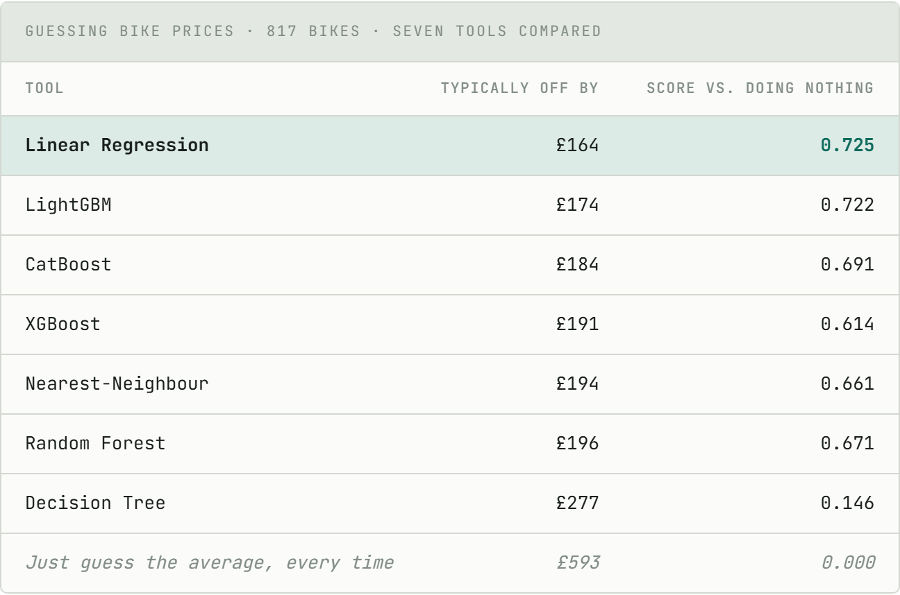
Linear Regression had the lowest MAE on this held-out split. The synthetic price formula includes non-linear depreciation and a few collector-bike outliers, so this result does not prove that bike pricing is truly linear. It shows that, with only 817 usable rows and this preprocessing, the simpler model generalised best according to the chosen KPI. LightGBM was close (£174 vs £164), while the single Decision Tree generalised poorly (R² 0.146).

MAE is the average absolute error in pounds. R² compares squared prediction error with a baseline that always predicts the test-set mean: 1 is perfect, 0 matches that baseline, and a negative value is worse.

Meet Larry

Larry always predicts the mean price (£1,174). R² = 0.725 means our model beats Larry by a wide margin. If you can't beat Larry, you don't have a model — you have an expensive average.

Side note: Random Forest ranked Distance_To_Service_Hub_KM third in importance — a column I invented with no real link to price. Don't trust feature-importance charts blindly.

Every run logged automatically. The straight line wins — but look how close LightGBM gets.

Phase 5 · Train: predict loan default

You are here: finance_features → classifier. Same train/test split pattern as Phase 4.

About 90% of the loans are repaid. A baseline that predicts “no default” for every application is therefore correct about 89.4% of the time, even though it catches no defaults:

def guess(applicant):
    return "will pay it back"   # every single time

When the important class is rare, accuracy is not enough on its own.

Classification KPIs: how we choose the useful model

The KPI comes from the cost of making the wrong decision. In this example, approving a loan that later defaults is more costly than sending a good application for additional review. That makes recall for the default class the primary KPI.

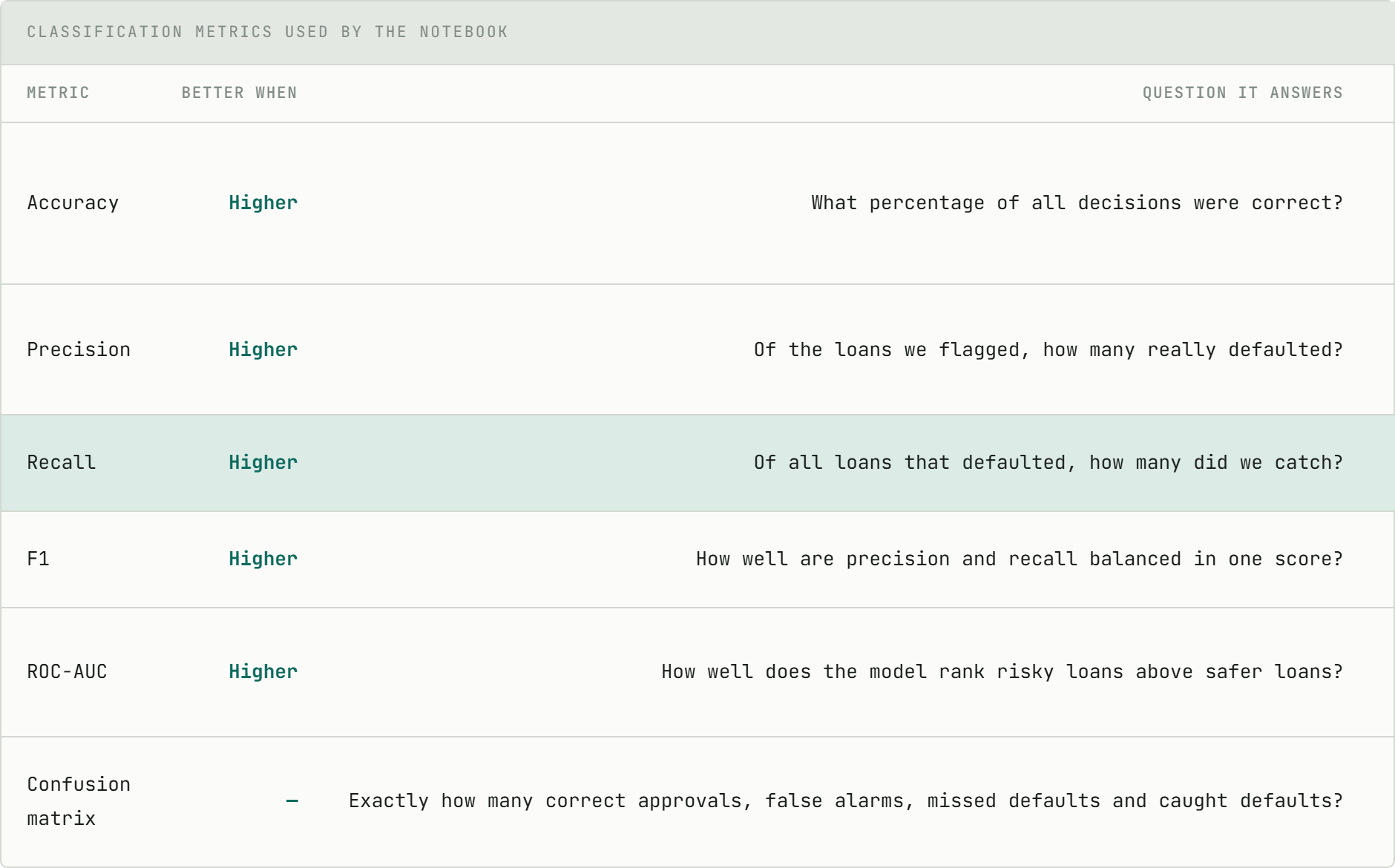
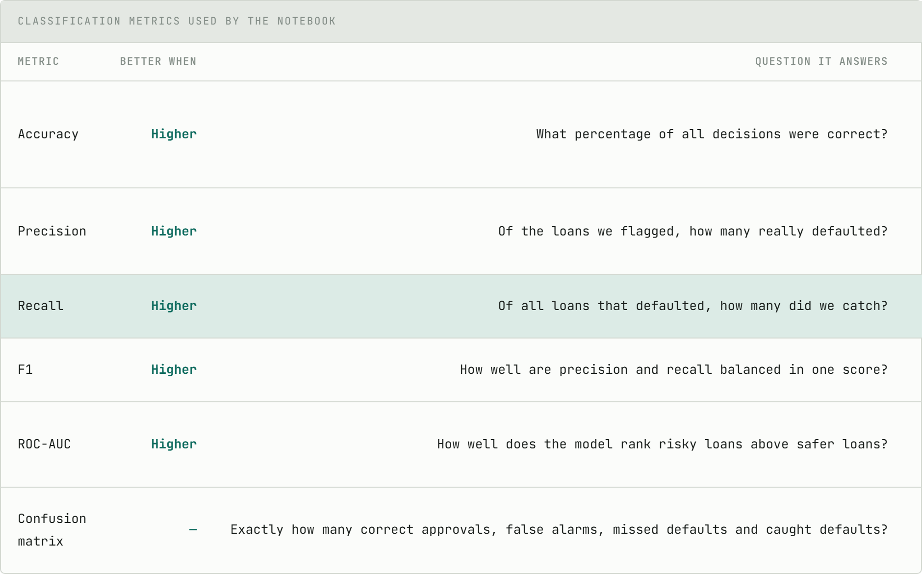
Selection rule: first require recall to improve substantially over the 0% baseline. Then check precision and the confusion matrix to confirm that the number of false alarms is operationally affordable. Finally, check ROC-AUC to confirm that the probability ranking contains useful signal.

Important limitation

The demo does not define a maximum review workload or an agreed financial cost for false positives and false negatives. For that reason, the balanced Random Forest is the selected demonstration model, not a production-approved winner. A production team should agree those limits before training and encode them as an acceptance gate.

The notebook trains on 32,000 rows and tests on 8,000 held-out rows. Of those test rows, 846 are defaults. It compares two Random Forest models:

default_model = RandomForestClassifier(
    n_estimators=100,
    max_depth=8,
    random_state=42,
)

balanced_model = RandomForestClassifier(
    n_estimators=100,
    max_depth=8,
    class_weight="balanced",
    random_state=42,
)
default_model.fit(X_train, y_train)
balanced_model.fit(X_train, y_train)

class_weight="balanced" gives more influence to the rare default rows during training. This produces a newly trained model; it is not the same fitted model with a different display threshold.

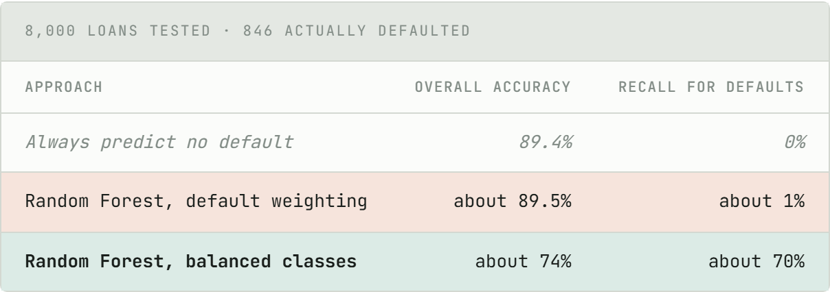
The exact figures are logged in MLflow, but the direction is clear: the default model catches only a handful of the 846 defaults, while the balanced model catches roughly seven out of ten. Its overall accuracy is lower because it also sends more good applications for review.

How selection works in the current notebooks

The notebooks log every candidate's metrics, then manually set best_name to Linear Regression or the balanced Random Forest. They do not automatically calculate a winner. That is acceptable for a transparent demo; a production workflow should turn the agreed primary KPI and guardrails into a repeatable selection and approval step.

The four boxes

Every prediction lands in one of four groups:

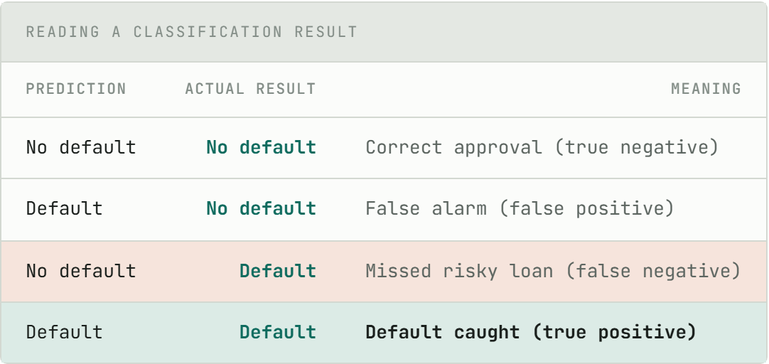
Precision asks: of the applications we flagged, how many really defaulted? Recall asks: of all applications that defaulted, how many did we catch? Improving recall usually creates more false alarms, so the final operating point is a business decision.

Worth remembering

For this use case, a lower-accuracy model can be more useful if it catches substantially more defaults. Report the confusion matrix, precision and recall alongside accuracy.

AUC: does the model rank risk well?

AUC asks whether a randomly chosen default is usually scored as riskier than a randomly chosen non-default. It uses probability scores rather than one fixed approval threshold. In this experiment both Random Forest variants are around 0.80 AUC, so both contain useful ranking signal even though their class predictions differ sharply.

AUC is useful, but it does not choose the business threshold for you. Log AUC together with precision, recall and the confusion matrix.

Phase 6 · Save and score

You are here: models selected → save the fitted model → load it from another notebook → score sample rows.

What the notebooks actually save

The training loop logs metrics to MLflow and attempts to register every non-baseline candidate with fe.log_model(). On this workspace, model artifact upload can fail even when the metrics were recorded successfully. The working handoff therefore saves only the selected model to a Unity Catalog Volume with joblib:

payload = {
    "model": best_model,
    "model_name": best_name,
    "feature_names": list(X_train.columns),
}
joblib.dump(payload, "/Volumes/pedalflow/ml/data/models/model.joblib")

Saving feature_names matters. The inference notebook uses that list to select the same columns in the same order and fails clearly if a required feature is missing.

Registry versions

If registration succeeds, a higher version number only means “saved later.” It does not mean the model is better. Promotion should be based on logged metrics and an explicit approval process.

What inference currently does

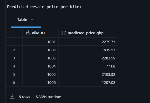
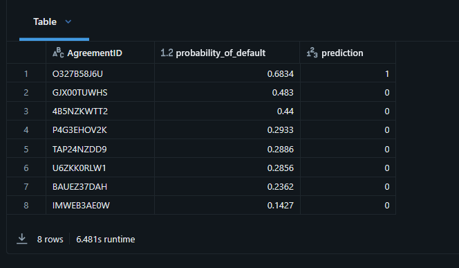
Each 03_inference.ipynb notebook loads the saved joblib payload, reads selected rows from the feature table, restores the expected column order and displays predictions. The classification notebook also displays probability_of_default.

payload = joblib.load(MODEL_PATH)
model = payload["model"]
expected = payload["feature_names"]

features = spark.table(FEATURE_TABLE).toPandas()
X = features[expected]
features["prediction"] = model.predict(X)

This proves that the artifact can be handed from training to inference. It is not yet a production batch pipeline: the current notebooks score a small sample and do not write ebike_predictions or finance_predictions tables. Real-time serving is also not implemented here.

What got built

Pulling the map from the top of this post back out, filled in with what actually exists in the workspace right now:

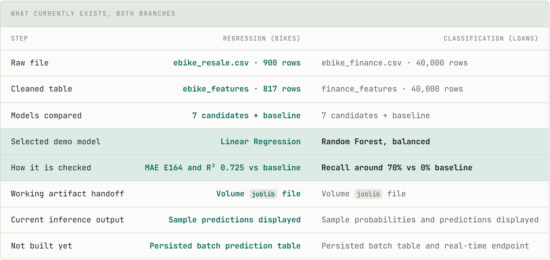
Two takeaways: the selected model is not always the fanciest algorithm, and the primary KPI must match the business question—not whichever number looks best after training.

Worked example: why 89.5% is not enough

Pipeline version — 8,000 rows, 846 corrupted, 7,154 clean:

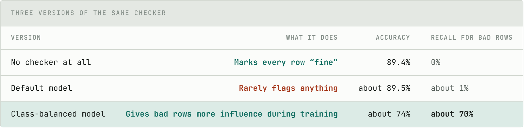
Step 1: Mark everything "fine" → 7,154/8,000 = 89.4% accurate, 0 catches. That's your floor.

Step 2: The default trained checker remains close to 89.5% accurate but catches only about 1% of corrupted rows. For the purpose of finding corruption, it barely improves on doing nothing.

Step 3: Retrain with class balancing. Accuracy falls to roughly 74%, but recall rises to roughly 70%. “Worse” accuracy, much better coverage of the problem.

Step 4: Same trap as a dashboard showing "99% rows OK" while missing the duplicate-key failures you built the job to find.

Rule

Rare target → ask of the bad rows, how many did we catch? Not "% correct overall."

Takeaways for your team

In standup terms:

• Feature engineering is most of the work. Nulls, encoding, scaling — same as building a gold table. model.fit() is two lines.

• Feature table = contract. Same columns, same order, same logic for train and score. Save to Unity Catalog.

• Log every run. MLflow metrics or you're arguing from notebook output.

• Version ≠ best. If registry upload succeeds, select versions by metrics and approval status—not by the highest number.

• Always report the baseline. Larry for regression, "always approve" for classification.

• Pin reproducibility. random_state=42, stratify=y — same reason you pin package versions.

• Batch vs real-time is infra, not ML. Know which you can support before promising it.

Code, data, and reproducible numbers: Machine-Learning-w-DBX.

Thanks for Reading .Keep in touch 👍